How Watts to Wills works

Start here for a guided tour of the model—no economics or engineering background required. For formulas, calibration choices, and implementation details, open the technical deep dive →. Watts to Wills is a tool for exploring possible futures, not predicting which one will happen. Close this guide with Esc.

1 · Start here

The controls are on the left and the results are on the right. Change a slider, choose a preset, or drag a chart point and the model updates immediately. The colored strip at the top gives the quickest summary: green means supply is keeping up; red means demand has moved ahead.

The name describes the journey the model follows. It begins with the electricity and computing equipment AI requires. It ends with the people and purposes that make the output valuable. Everything in between—capacity, access, prices, revenue, and ownership—shapes how much value is created and who receives it.

The defaults form one internally consistent scenario, not a “best guess.” Use them as a starting point, then change the assumptions that matter to you. Hover over controls for short explanations. Expand Model assumptions & provenance at the bottom for sources and evidence labels.

2 · What the model follows

Every update moves through the same chain:

1. How quickly people and organizations ask for more AI work.
2. How much electricity, equipment, and serving capacity are available.
3. Whether supply meets demand—and what happens to prices and access when it does not.
4. How much useful work the available output can support.
5. How revenue and broader economic gains are shared under the selected ownership and access rules.

Some parts feed back into one another. For example, broader gains can bring more people into effective use, which can create further gains. The model repeats those calculations until they settle on a stable result.

3 · Building supply

AI supply comes from two things working together: powered infrastructure and the amount of useful computing each watt can deliver. The model keeps track of when equipment entered service because newer systems can do more work with the same electricity.

Build-out is how much new powered capacity the industry tries to add. Power availability is how much can actually be connected and run. When power is tight, attempted projects may arrive late or not at all. Retired facilities return their grid connections to the available pool.

The per-watt capability growth control represents better chips, systems, and serving methods. The decommission age controls how long older equipment stays in the frontier fleet. Named presets are coherent stories about possible build paths, not announced construction schedules.

4 · Growing demand

The demand curve describes how quickly requested AI work grows each year. The default begins very quickly and slows over time. Because yearly growth compounds, small changes near the beginning can have large effects later.

Token efficiency represents getting the same useful result with less generated output. Context represents how much information a model must consider for each request. Longer context generally requires more computing. Sparse-attention adoption reduces that burden in the scenario.

Not every task requires the largest model. The tier table shows how work is divided among different serving classes. Capability drift moves eligible work toward smaller, cheaper classes as technology improves, while the persistent floor keeps some work in its original class. Local serving moves work onto user-owned devices: it still creates modeled value, but it no longer uses the datacenter fleet or generates provider revenue here.

5 · Shortages, prices & money

A crunch begins when requested computing exceeds available supply. The model then serves a smaller share of demand and raises its cost-based scenario prices. It applies the shortage proportionally; it does not decide that one user, task, or country goes first.

The price ladder compares the modeled cost of serving different classes of work. It is not a forecast of any provider's list price. Subscription revenue comes from covered personal users; other datacenter use is billed at the model's tier prices.

The cash-flow chart separates provider revenue from the cost of building and operating the fleet. Capital spending includes replacement equipment. Operating costs follow the powered footprint. Switching to % of GDP shows the same flows relative to the model's world-output path.

6 · Finding a no-crunch path

Solve: no crunch asks a practical counterfactual: how much capacity would the industry need to attempt if it wanted supply and demand to stay in balance? The solver leaves the 2026 build unchanged and begins responding in 2027. It still respects retirement and the selected power limits.

If the shortage is already unavoidable—or the grid cannot supply enough power—the model reports that constraint instead of pretending the past could have changed. Ramp limits let you impose a more gradual industrial response. They apply to the solver only, not to paths you draw yourself.

7 · Value created vs money earned

The model separates two questions that are often blended together:

• How much useful value is created? This is the modeled gain from work that can actually be delivered and put to use.
• How much money is captured? This is the modeled revenue, payments, and retained surplus recorded at scenario prices.

The two can move differently. A shortage may raise provider revenue while preventing useful work from being done. Cheaper serving may reduce revenue per unit while allowing far more work to happen. The value layer is intentionally visible as a set of assumptions; it is not a directly measured world total.

8 · From output to useful work

More AI output is not automatically more value. People and organizations need access, skills, attention, and worthwhile ends for that output. The model calls this bridge between produced output and useful outcomes mediation.

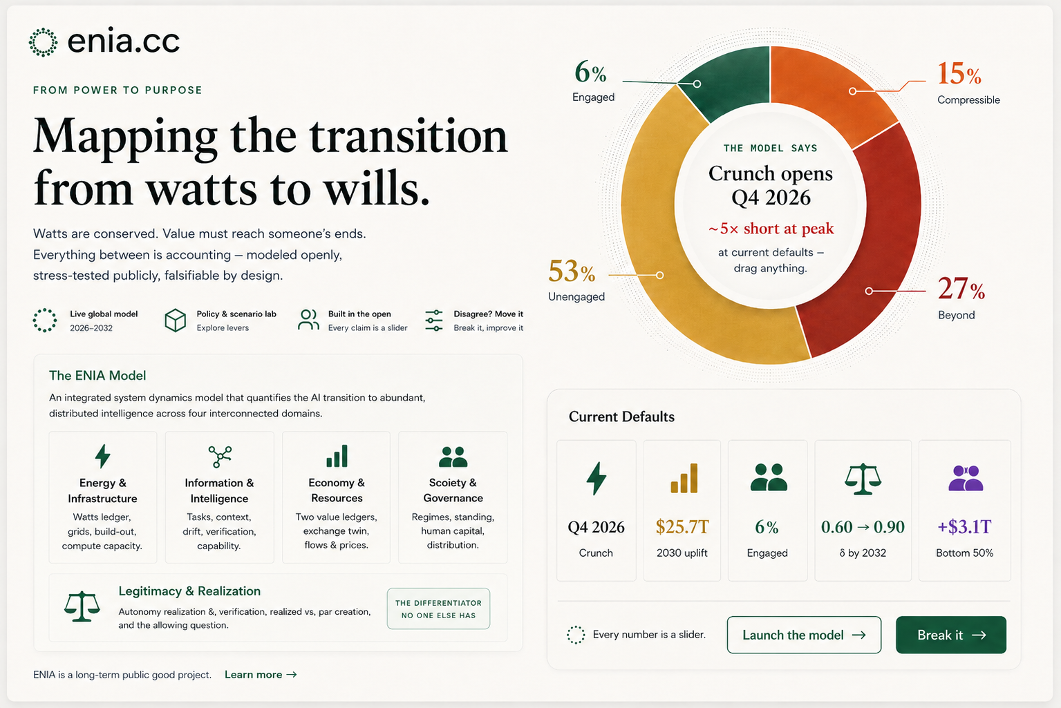
Work that fits within the modeled capacity of engaged users is treated as engagement-produced. Work produced beyond that envelope is treated as autonomy-produced. The δ control asks how much value the second kind realizes relative to the first, and how quickly that difference disappears.

The addressable-population controls ask how many adults can make intensive use of the technology and how that group grows as the economy changes. These are scenario assumptions, not headcounts or forecasts.

9 · Who benefits

The five regimes apply different rules to the same underlying economy:

• BAU extends current patterns of ownership, access, and pass-through.
• Enclosure concentrates access and keeps more gains with owners.
• Dividend returns part of captured value as equal cash payments.
• Basic compute provides access in kind and opens modeled use to everyone.
• Broad ownership shares a larger part of the capital stream across the population.

The tranche chart shows how people move among fixed resource bands. The regime frontier compares gains for the economy as a whole with gains for the bottom half. These are comparisons among explicit rule sets, not rankings of real policies.

When the human-capital ledger is on, earlier access can also affect learning, experience, and the ability to use later systems. Those relationships are sensitivity assumptions, not established causal estimates.

10 · Reading the charts

• Rationing strip and verdicts — when supply has room, when it becomes tight, and when the first crunch arrives.
• GDP effect by build-out path — how much modeled output changes under four named construction paths.
• The race and utilization — demand and supply on the same timeline, plus how fully the fleet is used.
• The watts ledger — the powered fleet grouped by age. Growing older bands show slower replacement.
• Fleet demand by tier — which serving classes account for the fleet's workload.
• Uplift by production mode — where modeled value comes from: billed engagement, local engagement, or autonomous production.
• The tranches — how the population is distributed across fixed resource bands by 2032.
• The regime frontier — how each ownership and access regime changes total gains and bottom-half resources.
• Price ladder and cash flows — modeled prices, revenue, construction costs, operating costs, and the gap between money and broader value.

11 · Things to try

• Ask what avoids a crunch. Keep the default demand path, press Solve: no crunch, then compare the required build with the selected power path.
• Test an infrastructure slowdown. Choose Capex winter and Committed power. Change the decommission age and watch older equipment occupy more of the fleet.
• Separate higher prices from lost value. Tighten power availability. Revenue may rise with scarcity even as less useful work is delivered.
• Compare cash with access. Switch between Dividend and Basic compute. Look at both the regime frontier and the 2032 tranche results.
• Test cheaper models. Turn capability drift off and on. Watch the gap between raw demand and compute-weighted demand.
• Stress longer tasks. Raise 2030 context and compare the cost pressure with the separate context-value assumption.

12 · What the model leaves out

Watts to Wills is intentionally broad, but it is not a complete economy. Important omissions include:

• Jobs and wages. It does not model displacement, employment, wage bargaining, or changes in labor supply.
• The supply of local devices. Local computing appears without competing for chips, electricity, or household budgets.
• A current global income map. The distribution baseline comes from an older stylized calibration and is best used for comparisons, not present-day estimates.
• Political feedback. Demand, ownership, access rules, and concentration do not change themselves in response to the results.
• Different priorities during shortages. The model reduces access proportionally rather than choosing winners and losers within a tier.
• Probability ranges. Sliders show sensitivity, but the model does not assign odds, confidence intervals, or a single expected outcome.
• Empirically settled value assumptions. Several links between output, useful work, growth, and human capability remain judgments to explore rather than measured laws.

13 · Plain-language glossary

• Crunch — the point when requested computing first exceeds available supply.
• Fleet — the powered datacenter equipment represented by the model.
• Compute unit — a common yardstick that lets different kinds of AI work be compared.
• GPU-equivalent — capacity expressed in units of today's reference accelerator.
• Footprint — the electricity used by the modeled frontier fleet.
• Capability drift — work moving to smaller, cheaper serving classes as they become capable enough.
• Local serving — work performed on user-owned devices rather than in the datacenter fleet.
• Creation — the model's estimate of useful economic gain.
• Capture — the money received by providers, owners, workers, or users.
• Mediation — the people, skills, attention, and access that turn output into useful outcomes.
• δ — how much value autonomous production realizes compared with work shaped through human engagement.
• Tranches — fixed resource bands used to compare distributional outcomes.

For exact equations, parameter definitions, solver behavior, calibration notes, and version history, continue to the technical deep dive →. For external sources and evidence labels, expand Model assumptions & provenance in the page footer.